Graph Databases for Beginners: Graph Search Algorithm Basics

(Neo4j Blog)←[:BACK]

By Joy Chao, Novice Graphista | August 1, 2016
 

While graph databases are certainly a rising tide in the world of technology, graph theory and graph algorithms are mature and well-understood fields of computer science.

In particular, graph search algorithms can be used to mine useful patterns and results from persisted graph data. As this is a practical introduction to graph databases, this blog post will discuss the basics of graph theory without diving too deeply into mathematics.

In this “Graph Databases for Beginners” blog series, we have covered why graphs are the future, why data relationships matter, the basics of data modeling, data modeling pitfalls to avoid, why a database query language matters, why we need NoSQL databases, ACID vs. BASE, a tour of aggregate stores, other graph data technologies and native versus non-native graph processing and storage.

Today’s discussion will be more theoretical, discussing different graph search algorithms and how they’re used, including Dijkstra’s algorithm and the A* algorithm.

Depth- and Breadth-First Search

There are two basic types of graph search algorithms: depth-first and breadth-first.

The former travel from a starting node to some end node before repeating the search down a different path from the same start node until the query is answered. Generally, depth-first is a good choice when trying to discover discrete pieces of information. They are also a good strategy for general graph traversals.

The most classic or basic level of depth-first is an uninformed search, where the algorithm searches a path until it reaches the end of the graph, then backtracks to the start node and tries a different path. On the contrary, dealing with semantically rich graph databases allows for informed searches, which conduct an early termination of a search if nodes with no compatible outgoing relationships are found. As a result, informed searches also have lower execution times.

(For the record, Cypher queries and Java traversals generally perform informed searches.)

Breadth-first algorithms conduct searches by exploring the graph one layer at a time. They begin with nodes one level deep away from the start node, followed by nodes at depth two, then depth three, and so on until the entire graph has been traversed.

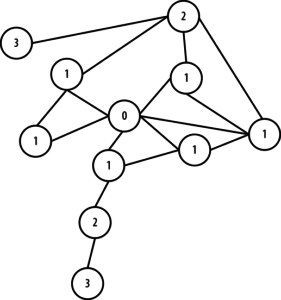
Dijkstra’s Algorithm

The goal of Dijkstra’s algorithm is to conduct a breadth-first search with a higher level of analysis in order to find the shortest path between two nodes in a graph. It does so in the following manner:

1. Pick the start and end nodes and add the start node to the set of solved nodes with a value of 0. Solved nodes are the set of nodes with the shortest known path from the start node. The start node has a value of 0 because it is 0 path-length away from itself.
2. Traverse breadth-first from the start node to its nearest neighbors and record the path length against each neighboring node.
3. Pick the shortest path to one of these neighbors and mark that node as solved. In case of a tie, Dijkstra’s algorithm will pick at random.
4. Visit the nearest neighbors to the set of solved nodes and record the path lengths from the start node against these new neighbors. Don’t visit any neighboring nodes that have already been solved, as we already know the shortest paths to them.
5. Repeat steps three and four until the destination node has been marked solved.

Dijkstra’s algorithm is very efficient as it works only with a smaller subset of the possible paths through a graph. After each node is solved, the shortest path from the start node is known and all subsequent paths build upon that knowledge.

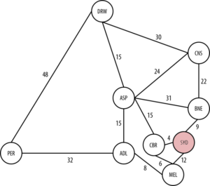
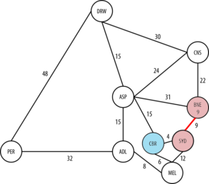
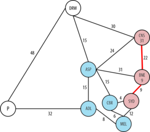
Dijkstra’s algorithm is often used to find real-world shortest paths, such as for navigation and logistics. Let’s see how it would find the shortest driving route between Sydney and Perth in Australia.



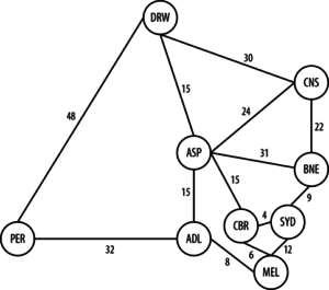
Sydney is the start node and is immediately solved with a value of 0 as we are already there.



Moving in a breadth-first manner, we look at the next cities a level away from Sydney: Brisbane, Canberra and Melbourne.



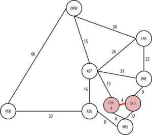
Canberra is the shortest path at 4 hours, so we count that as solved. We continue onto the next level, considering the next nodes out from our solved nodes and selecting the shortest paths. From there, Brisbane at 9 hours is the next solved node.



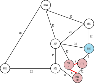
We move on, choosing between Melbourne, Cairns and Alice Springs. Melbourne is the shortest path at 10 hours from Sydney via Canberra, so it becomes the next solved node.



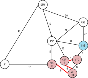
Our next options of neighboring nodes to solved ones are Adelaide, Cairns and Alice Springs. At 18 hours from Sydney via Canberra and Melbourne, Adelaide is the next shortest path.



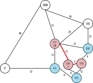
The next options are Perth (our final destination), Alice Springs, and Cairns. While in reality it would be most efficient to head directly to Perth, according to Dijkstra’s algorithm, Alice Springs is chosen because it has the current shortest path (19 total hours vs. 50 total hours). Note that because this is a breadth-first search, Dijkstra’s algorithm must first search all still-possible paths, not just the first solution that it happens across. This principle is why Perth isn’t immediately ruled out as the shortest path.



From Alice Springs, our two options are Darwin and Cairns. The latter is 31 hours to the former’s 34 hours, so Cairns is the next solved node.



The only unsolved node left from Cairns is Darwin.



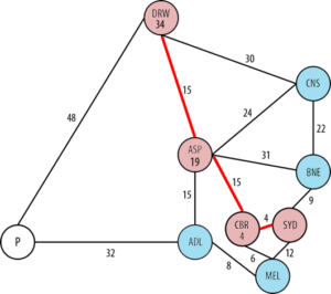
From Darwin, we make the final stretch and end up at Perth, with a cost of 82 hours for this given explored path.



Now that Dijkstra’s algorithm has solved for all possible paths, it can rightly compare the two routes to Perth:

• via Adelaide at a cost of 50 hours, or
• via Darwin at a cost of 82 hours

Accordingly, Dijkstra’s algorithm would choose the route via Adelaide and consider Perth from Sydney solved at a shortest path of 50 hours.

In the end, we can see that the algorithm uses an undirected exploration to find its results. Occasionally, this causes us to explore more of the graph than is intuitively necessary, as Dijkstra’s algorithm looks at each node in relative isolation and may end up following paths that do not contribute to the overall shortest path.

The example above could have been improved if the search had been guided by some heuristic like in a best-first search. To apply that in our own example, we could have chosen to prefer heading west over east and south over north, which would have helped avoid the unnecessary side trips taken.

The A* Algorithm

Consequently, the A* algorithm improves upon Dijkstra’s algorithm by combining some of its elements with elements of a best-first search. Pronounced “A-star”, the A* is based on the observation that some searches are informed, which helps us make better choices over which paths to take through the graph. Like Dijkstra’s algorithm, A* can search a large area of a graph, but like a best-first search, A* uses a heuristic to guide its search.

Additionally, while Dijkstra’s algorithm prefers to search nodes close to the current starting point, a best-first search prefers nodes closer to the destination. A* balances the two approaches to ensure that at each level, it chooses the node with the lowest overall cost of the traversal. As demonstrated by the example in the previous section, it is possible for Dijkstra’s algorithm to overlook a better route while trying to complete its search.

For more information on how the A* algorithm is used in practice, consult Chapter 7 of Graph Databases from O’Reilly media.

Conclusion

As has been illustrated above, graph search algorithms are helpful in traversing a set of graph data and providing relevant information. However, they also have their limitations. We have seen that there are many varieties of search algorithms, ranging from the more basic breadth-first and depth-first to uninformed and informed searches to the Dijkstra’s and A* algorithms. Each has its own strengths and weaknesses, no one type is better than another.


Ready to dive deeper into the world of graph databases? Learn how to apply graph technologies to real-world problems with O’Reilly’s Graph Databases. Click below to get your free copy of the definitive book on graph databases and your introduction to Neo4j.


Catch up with the rest of the Graph Databases for Beginners series:

• Graph Databases for Beginners: Why Graphs Are the Future
• Graph Databases for Beginners: Why Data Relationships Matter
• Graph Databases for Beginners: The Basics of Data Modeling
• Graph Databases for Beginners: Data Modeling Pitfalls to Avoid
• Graph Databases for Beginners: Why a Database Query Language Matters
• Graph Databases for Beginners: Why We Need NoSQL Databases
• Graph Databases for Beginners: ACID vs. BASE Explained
• Graph Databases for Beginners: A Tour of Aggregate Stores
• Graph Databases for Beginners: Other Graph Data Technologies
• Graph Databases for Beginners: Native vs. Non-Native Graph Technology

 

---